
Sales forecasts sit at the center of some of the biggest decisions a revenue team makes. Hiring plans. Territory coverage. Spend. Board expectations.
The challenge isn’t producing a number, but choosing a forecasting approach that fits how your sales motion works and the data you have today.
We’ll break down the most common sales forecasting methods, what each one is good at, where they fall short, and how to choose the right mix for your business.
Key Notes
- Time series and historical forecasting set a baseline for forecasting sales growth.
- Regression connects sales forecasts to measurable leading indicators and demand drivers.
- Stage and weighted pipeline methods quantify pipeline value using win probabilities.
- AI and multivariable models use behavior signals to predict revenue and flag risk.
The top 9 sales forecasting methods
These types of sales forecasting are not competing religions.
They are tools.
Some are baseline tools. Some are pipeline tools. Some are driver-based tools. Some require real data maturity.
To make this usable, each method includes:
- what it is
- what data it needs
- how it works
- a formula
- a concrete example
- when it fails
1) Time series analysis
Time series forecasting uses historical sales by time period to project the future by modeling patterns like trend and seasonality.
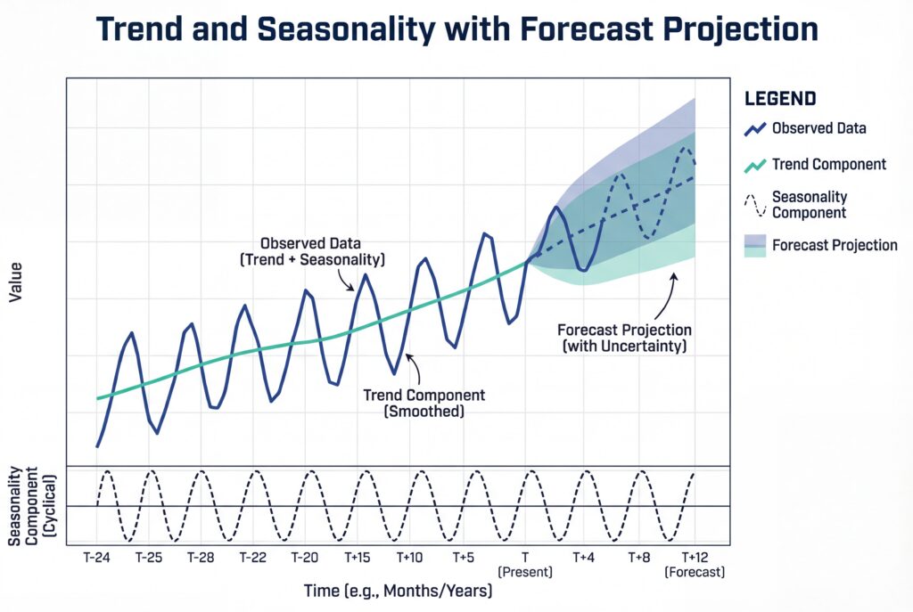
Why this matters:
CROs need a baseline that is not contaminated by current pipeline optimism. Time series gives you a “history-only” anchor.
Inputs needed:
A regular time series of past sales (monthly revenue is common), ideally 24+ months.
How it works:
- You plot sales over time
- Identify trend and seasonality
- Fit a model
- Then project forward
Simple versions are moving averages or exponential smoothing.
More advanced versions include ARIMA models.
Common formula (exponential smoothing):
Where:
- Ft = forecast for period t
- At−1 = actual in previous period
- α = smoothing factor between 0 and 1
Sales forecasting methods example:
- Last month actual revenue: $1,000,000
- Last month forecast: $950,000
- α = 0.3
Next month forecast:
F = 0.3 × 1,000,000 + 0.7 × 950,000 = 965,000
Works well when:
Sales have stable seasonality and enough history to trust patterns (mature subscription revenue, stable demand environments).
Fails badly when:
The business is in a regime change – new pricing, new motion, new market shock. Time series will confidently project the past into a future that no longer exists.
Note:
Time series is a baseline. It is not a commit forecast. Use it to catch delusion.
If your pipeline commit says 40% growth but the time series baseline says flat, you have something to inspect.
2) Regression analysis
Regression forecasting models sales as a function of one or more drivers, then uses those drivers to predict future sales.

Why this matters:
Some businesses are not “history-driven.”
They are “driver-driven.”
If pipeline and revenue move with leading indicators, regression gives you an early lens.
Inputs needed:
Historical sales paired with driver variables, such as marketing spend, qualified lead volume, pricing changes, or economic indicators.
How it works:
- You fit a model (often linear at first) to estimate coefficients.
- Then you forecast sales by plugging in expected driver values.
Formula:
Simple linear:
Y = β0 + β1 X + ε
Multiple drivers:
Y = β0 + β1X1 + β2X2 + ⋯ + Y
Sales forecasting methods example:
Say historical analysis suggests:
- β0 = 200,000
- β1 = 12 for “qualified leads”
If next month you expect 50,000 qualified leads:
- Y = 200,000 + 12 × 50,000 = 800,000
Works well when:
You have stable relationships between drivers and sales.
Often stronger in high-volume models where drivers are measured consistently.
Fails badly when:
You mistake correlation for causation, omit key variables, or overfit noise.
Also when relationships change over time. A new channel, a new pricing model, or a competitor entering can make your coefficients lie.
Note:
Regression is a discipline test. If you cannot agree on what drives sales, regression will expose that.
It also forces RevOps and Marketing Ops to align on leading indicators, not just activity volume.
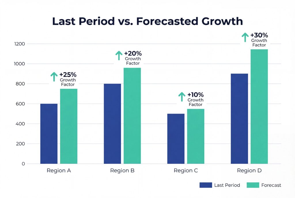
3) Historical forecasting
Historical forecasting projects the next period’s sales from past results, often applying a simple growth assumption.
Why this matters:
Every forecasting system needs a “quick baseline.” Historical forecasting is blunt, but it is fast and useful for sanity checks.
Inputs needed:
Periodic historical sales (12 to 24 months is typical).
How it works:
- Choose a baseline (last month, average of last 3 months, same month last year)
- Then apply a growth rate if relevant
Formula:
Forecast = LastPeriodSales × (1+GrowthRate)
Sales forecasting methods example:
- Last month closed: $500,000
- Average monthly growth last 6 months: 4%
Forecast:
- 500,000 × 1.04 =520,000
Works well when:
Demand is stable and you are not expecting step-changes.
Fails badly when:
Seasonality is strong or the business is in a transition.
“Next month equals last month” is not forecasting. It is a placeholder.
Note:
Treat this as a baseline and a test.
If your forecast deviates from historical baseline, you should be able to explain why in one sentence.
4) Opportunity stage forecasting
Opportunity stage forecasting assigns a win probability to each pipeline stage and sums the weighted value of open opportunities.

Why this matters:
This is the core pipeline-based forecasting method for many teams. When stages are real, it creates a forecast you can inspect deal by deal.
Inputs needed:
Open opportunities with stage and value, plus historical win rates by stage.
How it works:
- Define probabilities per stage (based on actual conversion, not opinion)
- Multiply each deal by its stage probability
- Sum the results
Formula:
Forecast = ∑i (DealValuei × WinProb(stagei))
Sales forecasting methods example:
- Deal A: $50,000 in “Demo” at 70% → $35,000
- Deal B: $80,000 in “Proposal” at 40% → $32,000
- Deal C: $120,000 in “Negotiation” at 60% → $72,000
Forecast total: $139,000
Works well when:
You have consistent stage definitions and you track stage conversion honestly.
Fails badly when:
Stages are not calibrated. If reps “move deals forward” to look good, stage probabilities become fiction.
Note:
Stage forecasting is only as good as stage integrity. If you fix one thing, fix stage definitions and enforcement.
It is hard work, but it pays for itself.
5) Weighted pipeline
Weighted pipeline forecasting is a simplified stage-weighted approach that often uses fixed stage percentages, sometimes based on judgement rather than conversion data.

Why this matters:
A lot of teams call this “forecasting” because it is easy to implement. It is better than guessing, but it’s also easy to abuse.
Inputs needed:
Open opportunities with stage and value, plus stage weights.
How it works:
Multiply each deal by a stage weight, sum the pipeline.
Formula:
Same structure as stage forecasting: ∑(DealValue × StageWeight)
Sales forecasting methods example:
If you set:
- Proposal = 50%
- Negotiation = 80%
Then:
- 10 deals at $10,000 in Proposal → $50,000 forecast
- 5 deals at $15,000 in Negotiation → $60,000 forecast
Total: $110,000
Works well when:
You are early and need a first-pass model, or you want a quick pipeline view for coverage checks.
Fails badly when:
You treat weights as permanent or you never update them.
It also fails when deal circumstances vary wildly within a stage.
Note:
Most teams over-trust this method. Accuracy often lands around 60 to 75% because it ignores deal-specific reality.
Use it as a lens, not a verdict.
6) Length of sales cycle forecasting
Length-of-cycle forecasting uses the age of a deal relative to the typical sales cycle to estimate close probability.

Why this matters:
Stage alone is not timing. Deal age adds a reality check. It helps you see stalled deals that “look late-stage.”
Inputs needed:
Historical average sales cycle length and deal age (days open) for current opportunities.
How it works:
- You calculate the average cycle length
- Then compare each deal’s age
Simple versions assume probability increases as time progresses.
Better versions use curves (survival analysis) to reflect stall risk.
Simple formula:
WinProb = min(1,DealAge/AvgCycle)
Sales forecasting methods example:
- Avg cycle: 90 days
- Deal age: 45 days
WinProb = 45/90 = 0.5
If deal value is $100,000, weighted value is $50,000.
Works well when:
Your sales cycle is relatively consistent by segment and product.
Fails badly when:
You have multiple motions mixed together (SMB and enterprise in one pipeline), or you have structural reasons deals can sit longer without being unhealthy.
Note:
This method is a truth serum for pipeline reviews.
If a deal is 2x your typical cycle length, you should not be debating probability. You should be debating whether it is real.
7) Intuitive or qualitative forecasting
Qualitative forecasting relies on human judgement and experience to estimate what will close and when.
Why this matters:
Some contexts do not have usable data. New product. New market. Very low volume.
In those contexts, pretending you have statistical certainty is worse than admitting you do not.
Inputs needed:
Rep and leader judgement, plus the core deal facts (buyer, timing, blockers, next step).
How it works:
Deals are assessed based on confidence, buyer signals, and deal narrative.
The discipline is in making the “why” explicit.
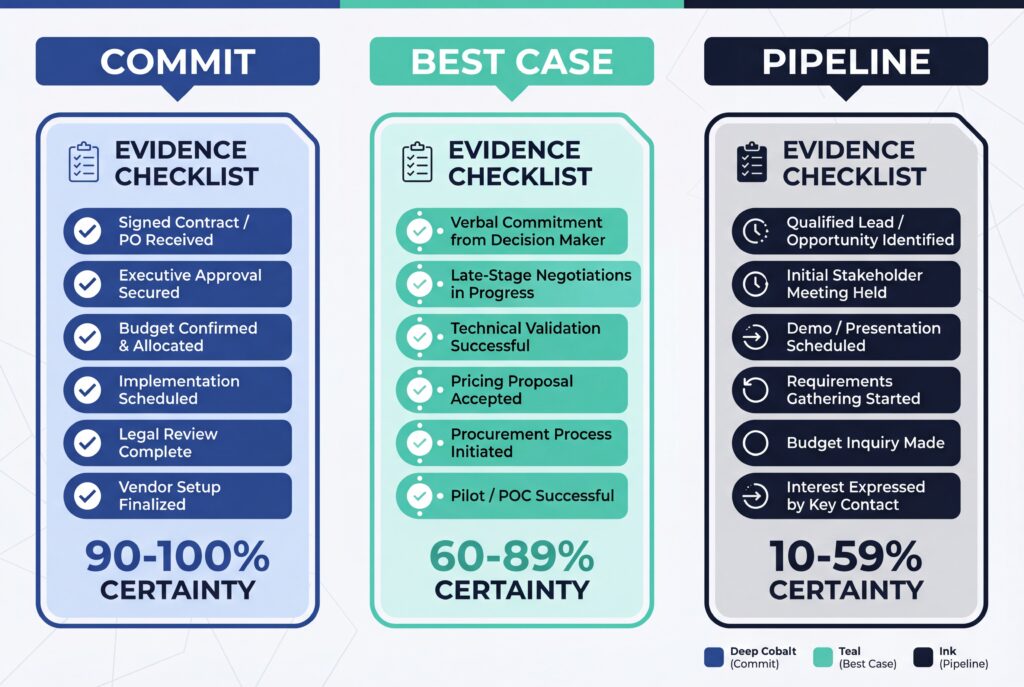
A practical structure (not a formula):
- Commit: clear mutual plan, buyer authority engaged, next step dated
- Best case: plausible but missing one core condition
- Pipeline: early, unclear, or unvalidated
Sales forecasting methods example:
A rep commits a deal because:
- Legal redlines are done
- Budget owner joined the last call
- Implementation date is agreed
- Next step is signature by Friday
That is not “gut feel.” That is an evidence-based judgement call.
Works well when:
- Data is sparse or the motion is new.
- Also works as a final inspection layer even in mature teams.
Fails badly when:
You let confidence replace evidence. Optimism bias will eat you alive.
Note:
Use qualitative forecasting as a layer, not the base.
If your forecast is purely judgement, your goal is to graduate out of that by building better inputs.
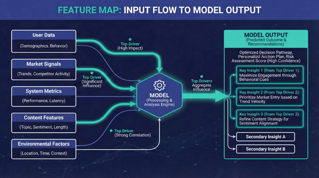
8) Multivariable analysis
Multivariable analysis uses many variables at once to forecast outcomes, capturing interactions that simple models miss.
Why this matters:
Stage, value, and close date are not the full story. Deal behavior matters. Engagement matters. Product usage signals matter.
Multivariable approaches let you incorporate those signals systematically.
Inputs needed:
A rich dataset of historical deals with multiple factors, such as stage history, activity levels, buyer engagement, lead source, segment, product, and timing.
How it works:
You model sales or win probability as a function of multiple variables, often using advanced regression or machine learning models.
The value is capturing interaction effects, like “late-stage + low engagement” being more dangerous than either signal alone.
Conceptual formula (multiple regression form):
Y = β0 + β1X1 + β2X2 + ⋯ + ε
In practice, teams may use models like random forests or gradient boosting to capture non-linear patterns.
Sales forecasting methods example:
A multivariable model might learn that win probability increases when:
- stage progression is consistent
- buyer engagement is high
- deal age is within normal range
And decreases when:
- next step dates slip repeatedly
- stakeholders disengage
- support or security reviews surface late
That gives you a forecast that looks more like real selling.
Works well when:
You have enough clean historical data and consistent instrumentation across teams.
Fails badly when:
You treat it like a magic bullet.
Without clean data and governance, multivariable models can perform worse than simpler methods. They can also become opaque if you do not build explainability in.
Note:
Complexity is not the win. Inspectability is.
If you cannot explain what variables drove a change, you will lose trust fast.
9) AI sales forecasting
AI sales forecasting applies machine learning to CRM and activity signals to predict revenue and deal outcomes by automatically weighting many inputs.

Why this matters:
AI can detect patterns humans miss, especially when signals interact (engagement timing, call outcomes, product usage spikes).
When data is disciplined, it can be a real advantage.
Inputs needed:
- CRM fields (amount, stage, close date, win/loss history)
- Sales engagement data (emails, calls, meetings)
- Marketing interactions
- Product usage
- Sometimes external signals
How it works:
- You label historical outcomes (won, lost, amount, timing)
- Train a model
- Then score live opportunities.
The model outputs a probability or expected value per deal and aggregates those into a forecast.
No single formula for AI sales forecasting:
AI learns the function. Under the hood, many tools blend time series, regression, and classification.
Sales forecasting methods example:
An AI model might output:
- Deal A: 80% win probability, $120,000 expected value
- Deal B: 25% win probability, $40,000 expected value
Then it sums expected values and flags risk factors (low engagement, slipping next steps, missing stakeholders).
Works well when:
You have a disciplined CRM culture and enough history. AI shines in data-rich environments.
Fails badly when:
Data is sparse or dirty. Bad close dates, missing activities, inconsistent stages. The model learns your mess.
Note:
AI does not replace leadership judgement. It replaces manual pattern detection. You still need humans to spot novel market shifts and to challenge assumptions.
How to choose the right sales forecasting method
Choosing a forecasting method is not a philosophical debate. It is a fit decision.
Here are the six factors that matter:
1) Sales cycle length
Short cycles stabilize quickly. Time series and simple baselines become useful.
Long cycles create timing risk. You need pipeline methods and often multivariable signals to avoid late-quarter surprises.
2) Deal volume
High volume smooths noise.
Low volume makes every deal matter, which raises the value of deal-level inspection.
3) Deal size concentration
If a handful of deals make the quarter, you need methods that expose deal health and risk drivers. Baselines will not protect you.
4) Data maturity
- 12 to 18 months gets you basic trend and simple pipeline weighting.
- 24+ months, with clean fields, opens up stronger time series and regression.
5) CRM discipline
If stage definitions are loose and close dates are never challenged, methods that depend on those fields will mislead you.
This is where “sales forecasting methodology” becomes real.
Your method is not just math. It is behavior enforcement.
6) Market volatility
When the market shifts, models that rely heavily on past patterns become fragile.
That is not a reason to abandon them.
It is a reason to run them alongside inspection and leading indicators.
A practical matching matrix

If you want one rule: start simple, then earn complexity.
The best way to forecast sales is usually a hybrid
Most teams do not need one method. They need a system.
A hybrid approach is how you avoid being held hostage by one set of assumptions.
The hybrid stack most teams should run
- Baseline forecast: Time series or historical growth to anchor expectations.
- Pipeline forecast: Stage-weighted, plus a sales-cycle overlay to catch timing risk.
- Inspection layer: Rep and leader judgement with explicit evidence.
That hybrid gives you three perspectives:
- What history suggests
- What current pipeline implies
- What humans see in the deal reality
When those disagree, that is not a problem. That is the signal.
How to combine outputs without creating chaos
The failure mode is running three models and letting everyone pick the one they like.
Instead, define a few forecast categories and stick to them:
- Commit
- Best case
- Pipeline
- Downside risk
Then require each category to be explainable by drivers you can inspect:
- stage conversion
- deal age and slippage
- engagement patterns
- missing stakeholders
- next step integrity
Where AI fits in a hybrid forecasting system
AI is strongest as a signal aggregator and risk detector.
It can surface patterns like:
- deals that progress stages but lose stakeholder engagement
- deals with repeated next-step slippage
- segments where conversion is deteriorating before revenue shows it
But AI only helps if the team actually runs on disciplined inputs. Otherwise you will get confident output that nobody trusts.
Frequently Asked Questions
What are the most common sales forecasting techniques used today?
Most teams combine multiple sales forecasting techniques, including historical forecasting, weighted pipeline, stage-based forecasting, and regression models. The most reliable forecasts usually blend a baseline method with pipeline and behavior-based inputs rather than relying on a single technique.
What’s the difference between sales forecasting methods and sales forecasting models?
Sales forecasting methods describe the approach or logic behind a forecast, like time series or pipeline-based forecasting. Sales forecasting models are the mathematical or statistical implementations of those methods, ranging from simple formulas to advanced machine learning models.
What is the best way to forecast sales growth for a scaling company?
The best way to forecast sales growth is to separate baseline growth from pipeline-driven growth. Use historical trends to anchor expectations, then layer in pipeline quality, deal timing, and leading indicators to model realistic upside and downside scenarios.
How accurate are sales forecasting methods in practice?
Accuracy varies widely by data quality and sales motion. Teams with disciplined CRM hygiene and clear stage definitions often reach 85–95% forecast accuracy, while teams without those foundations struggle regardless of the forecasting method they use.
Conclusion
Forecast accuracy doesn’t come from picking the “right” model, but from understanding what each sales forecasting method is good at and where it breaks.
Time series gives you a baseline. Pipeline methods show current exposure. Regression and AI surface drivers and risk patterns. None of them work in isolation, and none of them compensate for weak inputs.
The teams that forecast well are disciplined about data, ruthless about pipeline truth, and intentional about how methods are combined and inspected over time. That’s how forecasts become something leaders can explain, challenge, and rely on.
If you want to see how AI-driven analytics turn real pipeline behavior into defensible forecasts, start a free trial of EnableU’s Sales Excellence Platform and use it to connect pipeline health, deal intelligence, and revenue forecasting in one system.
Leave a Reply